We present our implementation of an Reinforcement Learning Algorithm called DeepDGP, presented by Lillicrap et al..
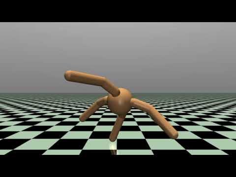
Trained MuJoCo environments
Introduction
- RL allows machines and software agents to automatically determine the ideal behavior within a specific context, in order to maximize its performance / rewards.
- Simple reward feedback is required for the agent to learn its behavior; this is known as the reinforcement signal.
Why DDPG?
-
Deep Q Network showed a great success in playing Atari games, however it works only for discrete action spaces.
-
Discretizing continuous action space with many dimensions suffers from curse of dimensionality.
-
DDPG solves this problem by introducing a variant of actor-critic method.
DDPG in Brief
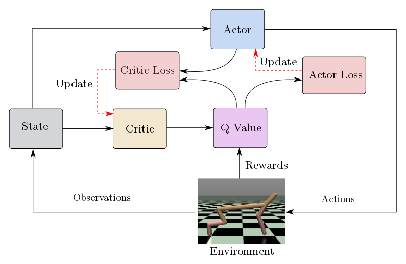
The agent consists of two neural networks namely actor and critic, which act as function approximator.
Actor tries to approximate the best policy which maps a state to optimal action, given by
\begin{equation} \mu (\theta^{\mu}): s_t \to a_t \end{equation}
Critic tries to approximate the predict the correct Q value, given by \begin{equation} Qc (\theta^{Qc}): s_t, a_t \to Q \end{equation}
We make a copy of each of the network and call them target networks. We use bellman equations and policy gradients to train actor and critic neural networks. Bellman equation given by,
\begin{equation} Q(s_t, a_t)^\pi = r_t + \gamma Q(s_{t+1}, a_{t+1})^\pi, \end{equation} where \(Q^\pi\) represents actual Q value.
Critic is trained using loss function given by
\begin{equation} L(\theta^{Qc}) = (Qc - y_t)^2, \end{equation}
where \(y_t\) is R.H.S. of bellman equation computed using the target networks.
Actor is trained by policy gradients which are given by,
\begin{equation} \frac{\delta Qc}{\delta \theta^{\mu}} = \frac{\delta Qc}{\delta a}\frac{\delta a}{\delta \theta^{\mu}}, \end{equation}
The parameters of target networks are updated slowly based on critic and actor, given by
\begin{equation} \theta^{Q’c} = \tau \theta^{Qc} + (1 - \tau)\theta^{Q’c} \end{equation}
\begin{equation} \theta^{\mu’} = \tau \theta^{\mu} + (1 - \tau) \theta^{\mu’} \end{equation}
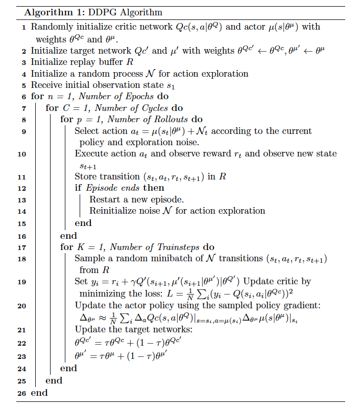
Algorithm
Hyper-Parameter Tuning
The classical trade-off faced by Reinforcement learning is Exploration vs Exploitation. This trade-off is adjusted by tuning the hyper-parameters of algorithm.
The hyper-parameters for DDPG are,
-
\(\gamma\) (Gamma) : Discount factor which determines the amount of importance given to future rewards compared to present.
-
Number of Roll-out steps : The number of steps after which networks are trained for K number of train steps. These are the steps allowed for random exploration experience build up.
-
Std Deviation of Action Noise : We use Ornstein-Uhlenbeck process for adding action noise, which suits to systems with inertia. By changing the deviation, we change the degree of exploration.
-
Number of Train steps : We train the parameters of Actor and Critic for K number of steps, after exploration steps.
Tuning the hyper-parameters for desired behaviors
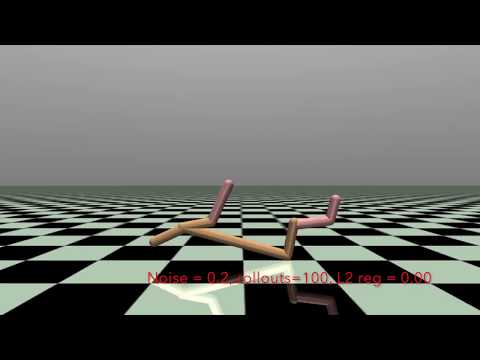
As an example, we see in Half-Cheetah environment, cheetah gets reward to run in forward direction. In the training, we find that it first flips itself as a result of initial random exploration and then behaves in a way to keep moving forward but in flipper state.
Also, as it flips initially or in between, its running speed gets affected causing reduction in overall reward.
We tackle this situation, by reducing number of roll-out steps, which are exploration steps causing it to flip at start. We see the changes in the algorithm reflected in the behavior of cheetah. Instead of rushing in forward direction, which would cause the loss of balance, cheetah learns a stable gait with increased speed and recieves overall maximum reward.
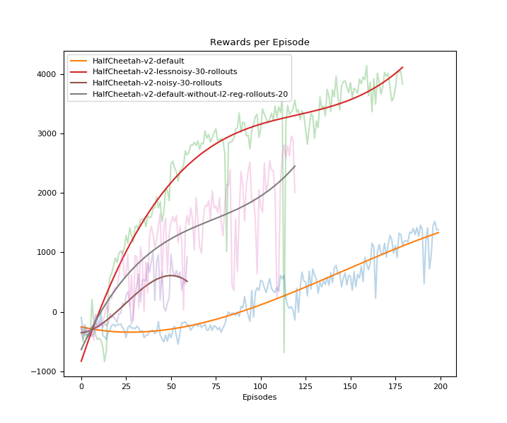
As it can be seen from images, the setting with less noise and less number of roll-out states with regularization receives the maximum reward and a plausible gait.
This video shows the effect of parameter tuning on the gait of Half Cheetah